Geospatial Analysis in R: getting started with the sf package

Last updated on Feb 21, 2019 6 min read R

The sf package is the successor to the common suite of geospatial analysis packages for R: sp, rgdal, and rgeos. This is a good thing because sf provides a unified solution to most of the geospatial operations that are often used within R.

The way you interact with spatial data in the sf universe is more intuitive than in the past because the structure of the sf class in R is very simple relative to the sp class. An object of the sf class consists of a normal data.frame with a geometry column that contains the geometry for each feature. That may not sound very exciting, but it makes for a much easier time when manipulating and summarizing spatial data.

If you are interested in the history and rationale for implementing the sf package, there are several enlightening blog posts and vignettes on the sf github page. I also found this guide very helpful for understanding the sf workflow.

Installation

Installing sf can be difficult while you align the system dependencies, but there are some steps outlined on the package readme that seem to work. The main system packages are GDAL, GEOS, PROJ. If your machine is already set up with geospatial software (e.g. QGIS) you probably have these installed already. For best results follow the installation instructions on github.

Fire it up

For this demo I am loading the tidyverse package which attaches my preferred set of data manipulation and visualization packages. I am also attaching the package ‘spData’ which contains some useful spatial datasets for demonstration.

library(tidyverse)

## Warning: package 'tibble' was built under R version 3.5.2

library(sf)
library(spData)

Download some data

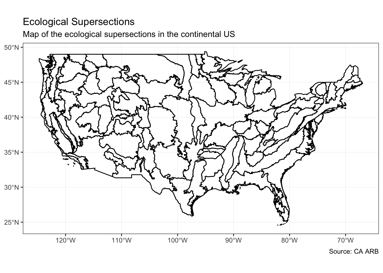
The ecological supersections make a cool spatial dataset that describe large ecological provinces across the continental US.

# import supersection shapefile
if (!file.exists("/tmp/gis-supersection-shape-file.zip")) {
  download.file(
    url = "https://www.arb.ca.gov/cc/capandtrade/protocols/usforest/2014/supersectionshapefiles/gis-supersection-shape-file.zip",
    destfile = "/tmp/gis-supersection-shape-file.zip"
  )
}

unzip(
  zipfile = "/tmp/gis-supersection-shape-file.zip",
  exdir = "/tmp/super"
)
superFile <- "/tmp/super/Supersections/Supersections.shp"

Reading in spatial data

The shapefile can be read in using the function st_read and projected to EPSG:4326 using the function st_transform. Notice that you can use pipes and the tidyverse framework on objects of the sf class! st_read can also handle alternative file formats such as geojson and GeoPackage (.gpkg).

supersectionShape <- st_read(dsn = superFile) %>%
  st_simplify(dTolerance = 2000) %>%
  st_transform(crs = 4326)

## Reading layer `Supersections' from data source `/private/tmp/super/Supersections/Supersections.shp' using driver `ESRI Shapefile'
## Simple feature collection with 95 features and 5 fields
## geometry type:  MULTIPOLYGON
## dimension:      XY
## bbox:           xmin: -2355031 ymin: 269687.9 xmax: 2257506 ymax: 3165565
## epsg (SRID):    NA
## proj4string:    +proj=aea +lat_1=29.5 +lat_2=45.5 +lat_0=23 +lon_0=-96 +x_0=0 +y_0=0 +datum=NAD83 +units=m +no_defs

Data structure

To understand why sf makes the world a better place, take a look at the class of supersectionShape. It’s an object of class sf and data.frame!

class(supersectionShape)

## [1] "sf"         "data.frame"

The data.frame structure of an sf object is also very convenient.

head(supersectionShape)

## Simple feature collection with 6 features and 5 fields
## geometry type:  GEOMETRY
## dimension:      XY
## bbox:           xmin: -123.5988 ymin: 42.08068 xmax: -98.82367 ymax: 48.99995
## epsg (SRID):    4326
## proj4string:    +proj=longlat +datum=WGS84 +no_defs
##          AREA PERIMETER    ACRES                 SSection SS_Name2
## 1 30741682875 1404657.1  7596137        Okanogan Highland     <NA>
## 2 28793819858 1201969.9  7114983       Northwest Cascades     <NA>
## 3 17147017863 3335379.1  4237070             Puget Trough     <NA>
## 4 21883664760  790723.2  5407398 Northern Rocky Mountains     <NA>
## 5 41675060546 1252913.5 10297621    Northern Great Plains     <NA>
## 6 69771019667 2634088.8 17240259           Columbia Basin     <NA>
##                         geometry
## 1 POLYGON ((-116.232 48.1383,...
## 2 POLYGON ((-122.846 44.13205...
## 3 MULTIPOLYGON (((-123.4378 4...
## 4 POLYGON ((-114.798 47.53692...
## 5 POLYGON ((-111.5483 47.1628...
## 6 POLYGON ((-118.4671 45.6895...

Plotting

sf objects can be plotted using base R plotting methods, but the ggplot method creates really nice looking maps with a familiar interface to many users.

ggplot() +
  geom_sf(
    data = supersectionShape,
    size = 0.5,
    color = "black",
    alpha = 0
  ) +
  theme_bw() +
  coord_sf() +
  labs(
    title = "Ecological Supersections",
    subtitle = "Map of the ecological supersections in the continental US",
    caption = "Source: CA ARB"
  )

Figure 1: Map of ecological supersections in continental US

Geospatial joins

Spatial joins operations (e.g. clip, overlay, etc) are very easy to perform in the sf framework. If two vector layers share the same projection, the function st_join can be used very effectively.

Let’s look at the relationships between ecological supersections and the US states. First, we need to make sure that the us_states sf object shares the projection EPSG:4326. We use the function st_crs for that.

st_crs(us_states)

## Coordinate Reference System:
##   EPSG: 4269 
##   proj4string: "+proj=longlat +datum=NAD83 +no_defs"

st_crs(supersectionShape)

## Coordinate Reference System:
##   EPSG: 4326 
##   proj4string: "+proj=longlat +datum=WGS84 +no_defs"

st_crs(us_states) == st_crs(supersectionShape)

## [1] FALSE

It does not share the same projection, so we are going to need to reproject before we perform any spatial joins.

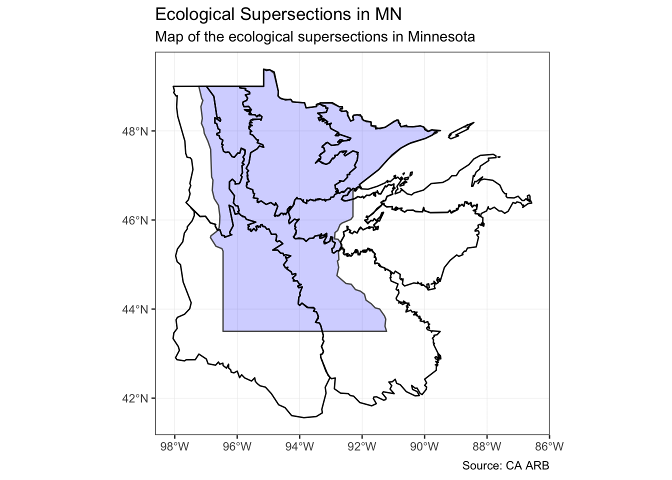
If we want to know which supersections are present in the state of Minnesota, we can perform a spatial join to answer that question. The type of join performed by st_join defaults to “intersect” (st_intersect), but can be set to one of these instead: st_disjoint, st_touches, st_crosses, st_within, st_contains, st_overlaps, st_covers, st_covered_by, st_equals, or st_equals_exact.

mnSupersections <- supersectionShape %>%
  st_join(
    st_transform(us_states, crs = 4326),
    join = st_intersects
  ) %>%
  filter(NAME == "Minnesota")

mn <- us_states %>%
  filter(NAME == "Minnesota")

ggplot() +
  geom_sf(
    data = mn,
    size = 0.5,
    fill = "blue",
    alpha = 0.2
  ) +
  geom_sf(
    data = mnSupersections,
    size = 0.5,
    color = "black",
    alpha = 0
  ) +
  theme_bw() +
  coord_sf() +
  labs(
    title = "Ecological Supersections in MN",
    subtitle = "Map of the ecological supersections in Minnesota",
    caption = "Source: CA ARB"
  )

Dissolving

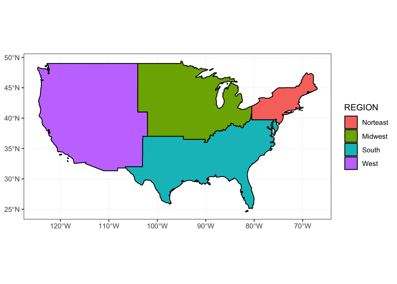
sf objects can be dissolved by common attributes if desired, or dissolved completely using the group_by and summarize logic from dplyr.

regions <- us_states %>%
  group_by(REGION) %>%
  summarize()

ggplot() +
  geom_sf(
    data = regions,
    aes(fill = REGION),
    size = 0.5,
    color = "black",
    alpha = 1
  ) +
  theme_bw() +
  coord_sf()

Bonus: working with rasters

Operations between rasters and sf objects are the same as before: load the raster using the raster package, summarize/extract raster data to vector layer using the extract function. Look for an update to this post once I see if there is a tidy way to summarize rasters within the piping framework!

# download low resolution climate rasters
if (!file.exists("/tmp/climate-rasts.zip")) {
  download.file(
    url = "http://biogeo.ucdavis.edu/data/worldclim/v2.0/tif/base/wc2.0_10m_tavg.zip",
    destfile = "/tmp/climate-rasts.zip"
  )
}

unzip(
  zipfile = "/tmp/climate-rasts.zip",
  exdir = "/tmp/climate-rasts"
)
rasts <- list.files(
  "/tmp/climate-rasts",
  full.names = TRUE
)

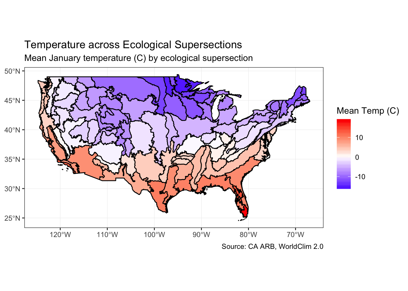
The climate rasters downloaded in the previous step represent the mean temperature by month at ~340 km2 resolution. For a real analysis, we would want the weighted mean temperature for each polygon (weighted on proportion of each raster cell falling within each polygon), but that takes a lot longer so we will just get the mean of intersecting cells.

janTemp <- raster::raster(
  rasts[grepl("tavg_01.tif", rasts)]
)

# reproject supersection shape to match raster
supersectionShape2 <- st_transform(
  supersectionShape,
  crs = raster::projection(janTemp)
)

# extract mean temp (C) for month of January for each polygon
janTemp <- raster::extract(
  janTemp,
  as(supersectionShape2, "Spatial"),
  fun = mean, weights = FALSE,
  na.rm = TRUE
)

supersectionShape2$janTemp <- janTemp

janPlot <- ggplot() +
  geom_sf(
    data = supersectionShape2,
    aes(fill = janTemp),
    size = 0.5,
    color = "black",
    alpha = 1
  ) +
  scale_fill_gradient2(
    high = "red", low = "blue",
    name = "Mean Temp (C)"
  ) +
  theme_bw() +
  coord_sf() +
  labs(
    title = "Temperature across Ecological Supersections",
    subtitle = "Mean January temperature (C) by ecological supersection",
    caption = "Source: CA ARB, WorldClim 2.0"
  )

Mapping mean temp in January confirms what we already knew: Minnesota is cold!

sf geospatial

Henry Rodman

biometrician

I am a forest biometrician based in Duluth, MN. My programming experience is primarily in R and python with a focus on processing geospatial data and statistical modeling. I have been working for SilviaTerra since June 2016. My primary responsibilities in the organization include building statistical models to predict forest attributes using remotely sensed data sources, and developing tools for analysis of forest inventory data.