Spatial data in R
vector data
There are several datasets built into the spData package that I will use:
us_statesworld
These are ‘simple features’ objects that are pre-loaded into R when you load the spData package. You can also load spatial data (shapefiles, geojson, etc) into R using the function st_read from the sf package. See my post on getting started with sf for more on that.
# us_states is a built in dataset to package spData
head(us_states)
## Simple feature collection with 6 features and 6 fields
## geometry type: MULTIPOLYGON
## dimension: XY
## bbox: xmin: -114.8136 ymin: 24.55868 xmax: -71.78699 ymax: 42.04964
## epsg (SRID): 4269
## proj4string: +proj=longlat +datum=NAD83 +no_defs
## GEOID NAME REGION AREA total_pop_10 total_pop_15
## 1 01 Alabama South 133709.27 [km^2] 4712651 4830620
## 2 04 Arizona West 295281.25 [km^2] 6246816 6641928
## 3 08 Colorado West 269573.06 [km^2] 4887061 5278906
## 4 09 Connecticut Norteast 12976.59 [km^2] 3545837 3593222
## 5 12 Florida South 151052.01 [km^2] 18511620 19645772
## 6 13 Georgia South 152725.21 [km^2] 9468815 10006693
## geometry
## 1 MULTIPOLYGON (((-88.20006 3...
## 2 MULTIPOLYGON (((-114.7196 3...
## 3 MULTIPOLYGON (((-109.0501 4...
## 4 MULTIPOLYGON (((-73.48731 4...
## 5 MULTIPOLYGON (((-81.81169 2...
## 6 MULTIPOLYGON (((-85.60516 3...# reproject to EPSG:4326
statesReproj <- us_states %>%
st_transform(4326)
worldReproj <- world %>%
st_transform(4326)raster data
Raster data can be loaded into R using the raster package. raster data objects do not play very nicely with sf objects, but that should change in the near future.
# download a climate raster
if (!file.exists("/tmp/climate-rasts.zip")) {
  download.file(
    url = "http://biogeo.ucdavis.edu/data/worldclim/v2.0/tif/base/wc2.0_10m_tavg.zip",
    destfile = "/tmp/climate-rasts.zip"
  )
}

unzip(
  zipfile = "/tmp/climate-rasts.zip",
  exdir = "/tmp/climate-rasts"
)
rasts <- list.files(
  "/tmp/climate-rasts",
  full.names = TRUE
)

janTemp <- raster::raster(
  rasts %>%
    stringr::str_subset("tavg_01.tif")
)
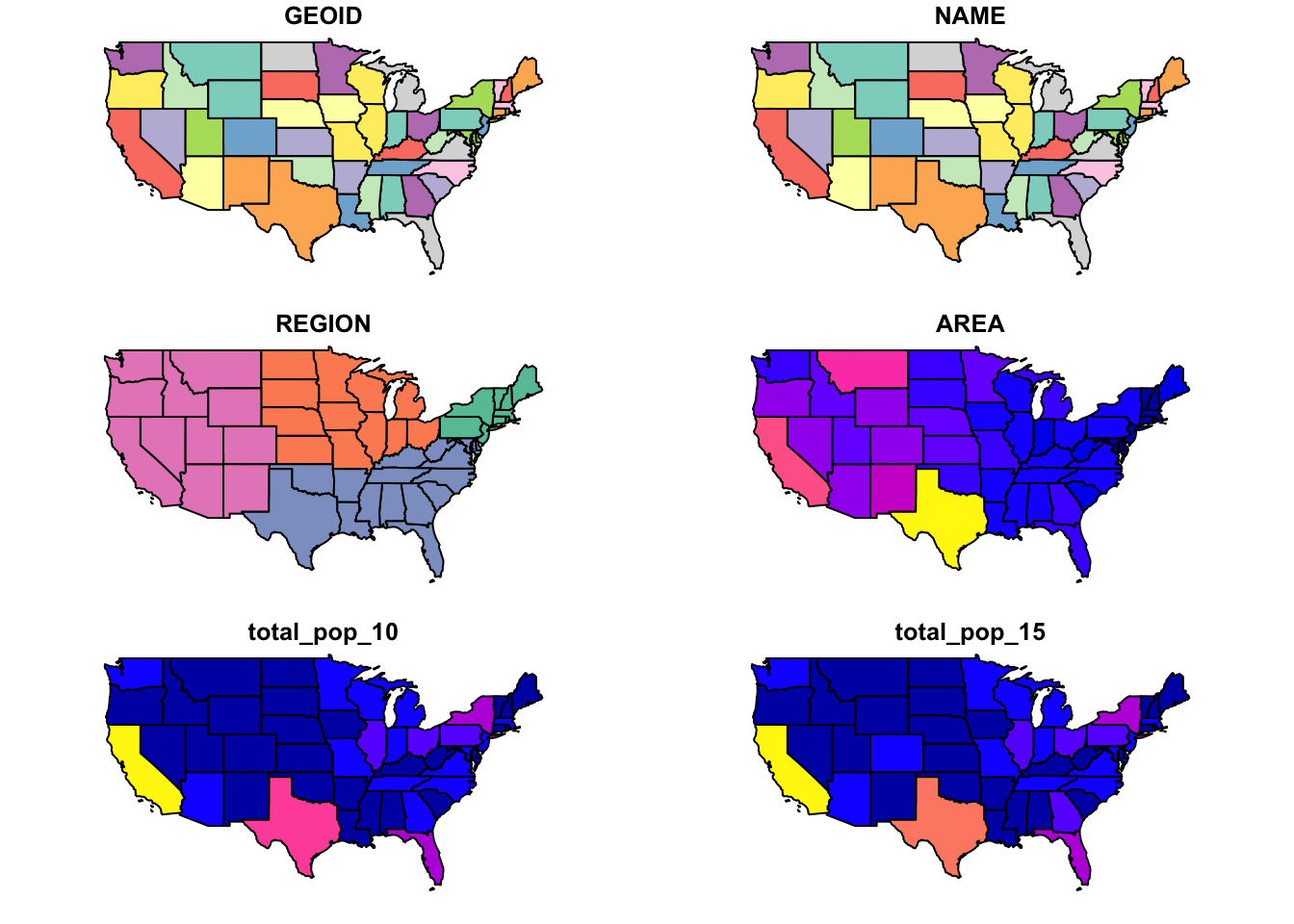
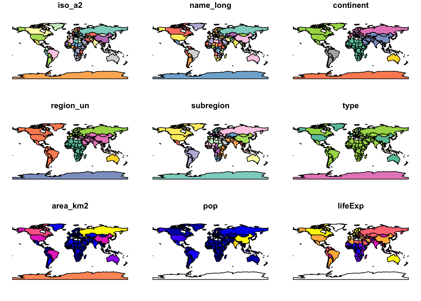
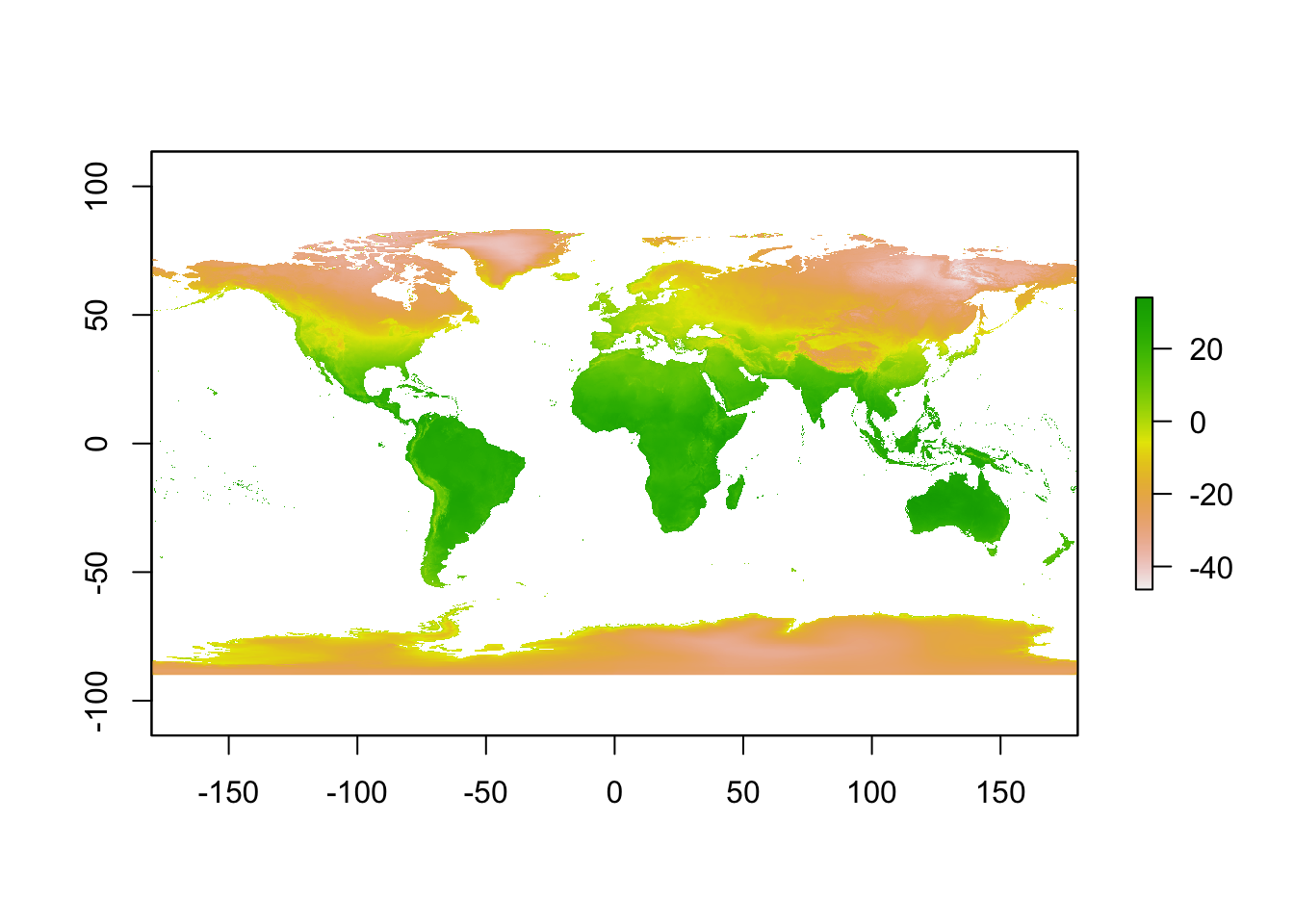
R and the spatial packages have easy methods for plotting spatial data.
plot(statesReproj)
plot(worldReproj)## Warning: plotting the first 9 out of 10 attributes; use max.plot = 10 to
## plot all
raster::plot(janTemp)
Leaflet
Leaflet is a powerful tool that allows you to render interactive maps with vector and raster layers. These maps can be embedded on websites or on static html documents generated by Rmarkdown (that’s how I made this post).
temp_pallette <- colorNumeric(
  c("#0C2C84", "#41B6C4", "#FFFFCC"),
  raster::values(janTemp),
  reverse = FALSE,
  na.color = "transparent"
)

# set extent of map to entire earth
world_extent <- worldReproj %>%
  mutate(planet = "Earth") %>%
  group_by(planet) %>%
  summarize() %>%
  st_convex_hull()

bounds <- st_coordinates(world_extent) %>%
  as_tibble() %>%
  setNames(c("lon","lat", "l1", "l2"))

leaflet(height = "500px") %>%
  addTiles() %>%
  addProviderTiles("Esri.WorldImagery") %>%
  addRasterImage(
    janTemp,
    color = temp_pallette,
    opacity = 0.8,
    group = "January mean temp (C)"
  ) %>%
  addPolygons(
    data = worldReproj,
    stroke = TRUE,
    weight = 2,
    smoothFactor = 0.2,
    fillOpacity = 0,
    color = "black",
    group = "countries"
  ) %>%
  addPolygons(
    data = statesReproj,
    stroke = TRUE,
    weight = 1,
    smoothFactor = 0.2,
    fillOpacity = 0,
    color = "blue",
    group = "states"
  ) %>%
  addLayersControl(
    overlayGroups = c(
      "January mean temp (C)",
      "countries",
      "states"
    ),
    options = layersControlOptions(collapsed = FALSE)
  ) %>%
  addLegend(
    pal = temp_pallette,
    values = raster::values(janTemp)
  ) %>%
  fitBounds(min(bounds$lon), min(bounds$lat), max(bounds$lon), max(bounds$lat))
## Warning in rgdal::rawTransform(projfrom, projto, nrow(xy), xy[, 1], xy[, :
## 106 projected point(s) not finite
## Warning in rgdal::rawTransform(projfrom, projto, nrow(xy), xy[, 1], xy[, :
## 106 projected point(s) not finite
## Warning in rgdal::rawTransform(projfrom, projto, nrow(xy), xy[, 1], xy[, :
## 106 projected point(s) not finiteGeopackages
Since I use open source software for everything, I disdain geodatabases! I understand why people use them but I am not able to open most geodatabases on my Mac or Linux machines. Fortunately there is an alternative to the geodatabase: the geopackage.
Geopackages can hold polygon, point, line, and raster layers (with tiles!). It is very easy to write vector layers to a geopackage from R, not as easy to write raster layers but it is possible (stay tuned).
# add countries layer
st_write(
  worldReproj,
  layer = "countries",
  driver = "GPKG",
  dsn = "open_source_gis.gpkg",
  delete_dsn = TRUE
)
## Deleting source `open_source_gis.gpkg' using driver `GPKG'
## Writing layer `countries' to data source `open_source_gis.gpkg' using driver `GPKG'
## features: 177
## fields: 10
## geometry type: Multi Polygon# add states layer
st_write(
statesReproj,
layer = "states",
driver = "GPKG",
dsn = "open_source_gis.gpkg",
update = TRUE
)## Updating layer `states' to data source `open_source_gis.gpkg' using driver `GPKG'
## features: 49
## fields: 6
## geometry type: Multi Polygon