The application of statistical survey sampling techniques to the assessment of forest resources (aka forest inventory) has been elemental to improvements in forest management practices across the globe. Sampling methods that can efficiently yield accurate and precise estimates are preferred by forest managers because collecting forest inventory data is difficult and expensive!
Two-stage sampling is useful in forest inventory because it can improve efficiency by reducing the number of stands (primary sample units) that are visited and by using auxilliary information for selecting sampled stands. This official name for this type of sample design is an unequal probability without replacement, two-stage sample. Unequal probability sampling is well documented in statistical textbooks, but the estimators for sample variance are much more complex than those for sample designs with equal probability and/or with replacement.
The Horvitz-Thompson estimators provide the framework for unequal probability sampling, but they need to be extended slightly to account for the variance from the second stage (sample variance within primary sample units). In fact, the Horvitz-Thompson estimators are sound for most design-based probability samples and can be reduced to the most commonly referenced equations for more ubiquitous sampling methods (e.g. simple random sampling with replacement).
The inspiration for this exercise was my struggle to compute inclusion probabilities for a sample drawn without replacement. Many references describe the computational complexity of obtaining the unconditional probability of inclusion for an element but do not provide an example or a reliable approximation, so I have devised a brute force simulation approach to estimating those probabilities.
Objectives
Let’s say that I am a forest manager that needs an estimate of the volume of standing trees in a tract of forest land. I want to obtain an accurate estimate for the lowest price possible. I am willing to pay more for a more precise estimate, but do not need an estimate that is more precise than +/- 10% at 90% confidence. In statistical terms, I would like the half-width of the 90% confidence interval to be roughly 10% of the estimate of the total volume.
Simulate the population
The forest is composed of 100 stands of forest that vary in size, most of the stands are Douglas-fir plantations. In general, we expect that older stands have greater volume stocking than young stands. We will randomly assign an age, size in acres, coefficient of variation of volume within the stand, then assign the mean cubic feet per acre for the stand.
# simulate a population of stands
stands <- tibble(id = 1:100) %>%
mutate(
acres = runif(
n = 100, min = 10, max = 200
),
age = runif(
n = 100, min = 10, max = 150
),
cv = runif(n = 100, min = 10, max = 100)
) %>%
mutate(
cuftPerAc = 3000 *
1 / (1 + exp(-(age - 40) / 15)) +
rnorm(n = 100, mean = 0, sd = 300),
cuftPerAc = ifelse(cuftPerAc < 0, 0, cuftPerAc),
cuftTot = cuftPerAc * acres
)
totalAcres <- sum(stands$acres)
totalCuft <- sum(stands$cuftTot)
meanCuft <- totalCuft / totalAcres
truth <- tibble(
source = "truth",
totalCuft = totalCuft,
meanCuft = meanCuft
)
stands %>%
ggplot(aes(x = age, y = cuftPerAc)) +
geom_point() +
ylab(bquote("volume (" ~ ft^{3} ~ "/ac)")) +
labs(caption = "volume over age for the forest")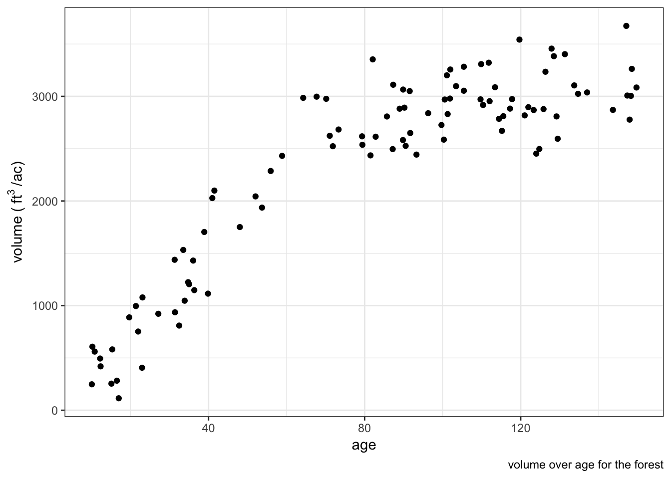 The true population mean stocking is 2336 cubic feet per acre, the population total is 2.326763110^{7} cubic feet!
Designing a two-stage sample
There are many ways to obtain an estimate of the total volume for the forest. The most expensive way would be to visit every tree in the forest, measuring several dimensions and estimating volume for every single tree. This would provide us with an accurate and precise estimate but would be time consuming and prohibitively expensive. We could also just guess the total based on what we know about the property. This would be very cheap today, but our estimate is likely to be inaccurate and will probably result in significant costs related to bad information down the road. Our best bet is to take a sample from the population. A simple random sample of 1/15 acre circular plots distributed across the property would be a fine way to sample the property, but traveling to each sample point could be very inefficient and we also want information about individual stands for planning purposes. We should do something besides a simple random sample.
A two-stage sample is an appealing option because we can obtain an accurate estimate of the population total while obtaining stand-level estimates that we will use for modeling forest growth and evaluating forest management options. We can also improve the precision of our estimates by sampling stands with weights that we expect to be correlated with our variable of interest (total volume).
Selecting stands
The population of stands could be sampled randomly, but since we are trying to obtain an estimate of total volume for the property, we need to make sure that we sample the stands that a) contribute the most to the total volume, and b) contribute the most variance to the population. Using the Horvitz-Thompson estimators, we can sample the stands however we want so long as we know the probability of each stand being included in the sample! This is a case of unequal probability sampling and the Horvitz-Thompson estimators will be statistically efficient if the probability of inclusion for each primary sampling unit is correlated with the variable of interest. In this case, we are going to weight our sample on age x acres since we believe the oldest stands are going to have the greatest stocking, and that the largest stands have the greatest total volume.
Inclusion probability
Some references approximate using where is the sampling weight for the th primary sample unit. This works fine when sampling with replacement, but sampling without replacement is slightly more complicated. The probability of including the th element on the th draw depends on the elements that were drawn in all draws . The distinction between and is very important. Think of as the likelihood of including the th element unconditional on the other elements selected in the sample. This can be calculated by computing the proportion of all possible samples where an element is selected but that sounds very difficult. Instead we will use the power of simulation to obtain an approximation of for each stand.
For this sample we are going to weight our sample on age * acres since we believe the oldest stands are going to have the greatest stocking, and that the largest stands have the greatest total volume. We have decided that we are going to sample 20 stands and install either one plot per 8 acres or 30 plots per stand, whichever is fewer.
stands$prop <- (stands$age * stands$acres) /
  sum(stands$age * stands$acres)

stands %>%
  ggplot(aes(x = age * acres, y = cuftTot)) +
  geom_point() +
  ylab(bquote("total volume (" ~ ft^{3} ~ ")"))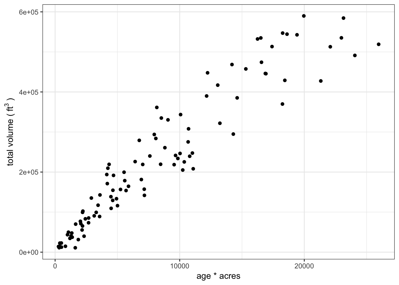
We need to estimate the inclusion probabilities () for all stands as well as the joint inclusion probabilities () for all pairs of stands. We can accomplish this with a simulation.
simulate_sample <- function(sims = 10000, stands, n, weight_var,
id_var, cores) {
weight_var <- enquo(weight_var)
id_var <- enquo(id_var)
allIds <- stands %>% pull(!! id_var)
simFrame <- bind_rows(
parallel::mclapply(1:sims,
function(i, ...) {
stands %>%
sample_n(n, weight = !! weight_var)
},
mc.cores = cores
),
.id = "sim"
)
sampledIds <- simFrame %>% pull(!! id_var)
if (!all(allIds %in% sampledIds)) {
missing <- allIds[!allIds %in% sampledIds]
warning(
paste0(
"these elements that were not included in any sample: ",
paste(missing, collapse = " ")
)
)
}
list(
simFrame = simFrame,
sims = sims,
n = n,
ids = allIds
)
}
estimate_pi_i <- function(simList, id_var) {
id_var <- enquo(id_var)
simList[["simFrame"]] %>%
group_by(!! id_var) %>%
summarize(pi_i = n() / simList[["sims"]]) %>%
select(!! id_var, pi_i)
}
estimate_joint_probs <- function(simList, id_var, pairs = NULL, cores) {
id_var <- enquo(id_var)
if(is.null(pairs)) {
ids <- simList[["ids"]]
idxs <- 1:length(ids)
pairs <- combn(ids, m = 2, simplify = FALSE)
} else {
ids <- unique(unlist(pairs))
idxs <- 1:length(ids)
}
estimate_joint_prob <- function(pair, simFrame, sims, cores, id_var) {
simFrame %>%
filter(!! id_var %in% pair) %>%
group_by(sim) %>%
mutate(n = n()) %>%
filter(n > 1) %>%
ungroup() %>%
select(sim) %>%
distinct() %>%
tally %>%
rowwise() %>%
mutate(
id1 = pair[1], id2 = pair[2],
row = idxs[which(ids == id1)],
col = idxs[which(ids == id2)],
jointProb = n / sims
) %>%
select(-n)
}
f <- bind_rows(
parallel::mclapply(
pairs,
estimate_joint_prob,
simFrame = simList[["simFrame"]],
id_var = id_var,
sims = simList[["sims"]],
mc.cores = cores
)
)
frame <- matrix(NA, nrow = length(ids), ncol = length(ids))
frame[as.matrix(f[3:4])] <- f$jointProb
frame[as.matrix(f[4:3])] <- f$jointProb
output <- data.frame(frame)
row.names(output) <- ids
names(output) <- ids
return(output)
}
simList20 <- simulate_sample(
sims = 10000,
stands = stands,
n = 20,
id_var = id,
weight_var = prop,
cores = 2
)
sampleSim20 <- estimate_pi_i(simList = simList20, id_var = id)
jointProbs <- estimate_joint_probs(
simList = simList20,
id_var = id,
cores = 2
)
sampleSim20 %>%
left_join(stands) %>%
mutate(pi_i_approx = 20 * prop) %>%
ggplot(aes(x = pi_i_approx, y = pi_i)) +
geom_point() +
geom_abline() +
xlim(0, 1.2 * max(sampleSim20$pi_i)) +
ylim(0, 1.2 * max(sampleSim20$pi_i)) +
xlab(bquote("approximate" ~ pi[i])) +
ylab(bquote("simulated" ~ pi[i]))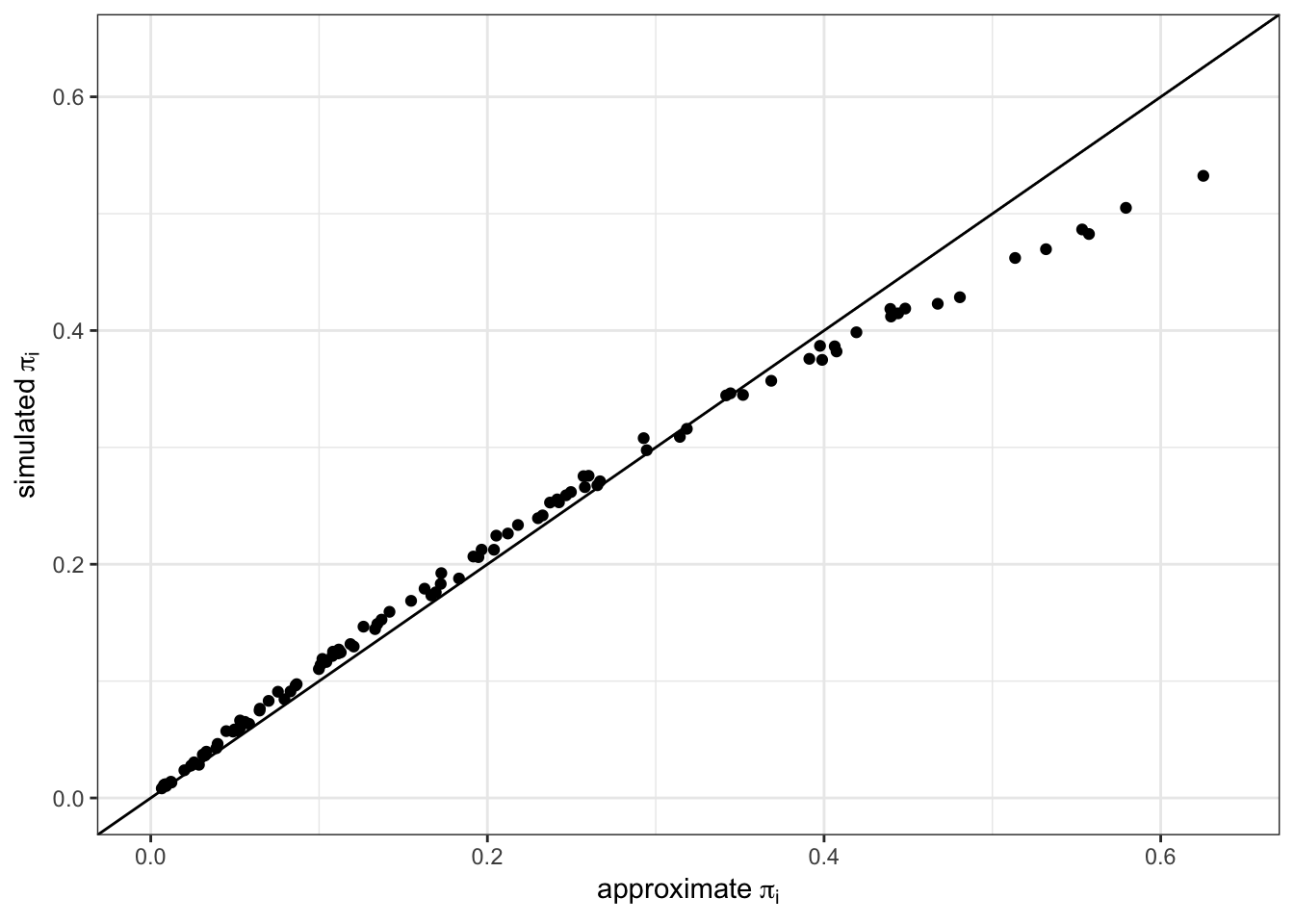 As you can see, there are subtle differences between the approximate values and the values generated from 10,000 simulated samples. We will use the simulated values for the rest of the analysis.
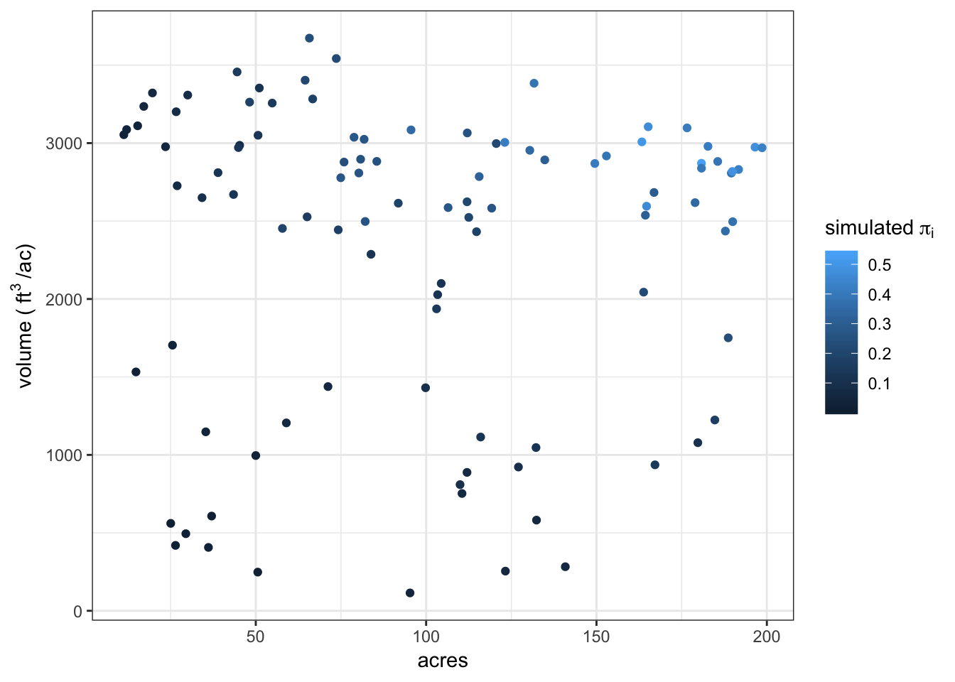
By plotting with the true total volume we can see that large stands with high volume stocking have the highest probability of inclusion in a sample of 20 stands.
sampleSim20 %>%
  left_join(stands) %>%
  ggplot(
    aes(
      x = acres,
      y = cuftPerAc,
      color = pi_i)
    ) +
  geom_point() +
  ylab(bquote("volume (" ~ ft^{3} ~ "/ac)")) +
  scale_color_continuous(
    name = bquote("simulated" ~ pi[i])
  )
sampleSim20 %>%
  left_join(stands) %>%
  ggplot(
    aes(
      x = pi_i,
      y = cuftPerAc * acres
    )
  ) +
  geom_point() +
  ylab(bquote("total volume (" ~ ft^{3} ~ ")")) +
  xlab(bquote("simulated" ~ pi[i]))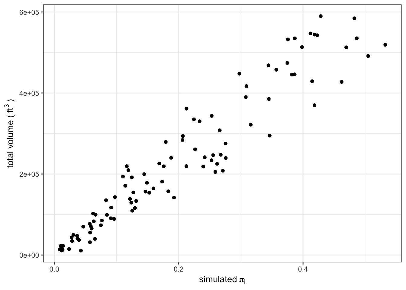
Example sample
Now we are going to step through a sample of the population.
acresPerPlot <- 6

sampStands <- stands %>%
  sample_n(size = 20, weight = prop) %>%
  group_by(id) %>%
  mutate(
    nPlots = max(
      2,
      min(ceiling(acres / acresPerPlot), 30)
    )
  ) %>%
  left_join(
    sampleSim20 %>%
      select(id, pi_i),
    by = "id"
  ) %>%
  ungroup()

stands %>%
  mutate(
    sampled = case_when(
      id %in% sampStands$id ~ "yes",
      ! id %in% sampStands$id ~ "no"
    )
  ) %>%
  ggplot(
    aes(x = acres, y = cuftPerAc, color = sampled)
  ) +
  geom_point() +
  ylab(bquote("volume (" ~ ft^{3} ~ "/ac)"))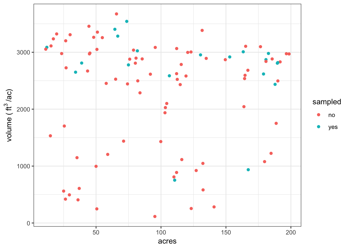
Measure plots
In each sample stand we are installing a systematic random sample of 1/15 acre circular plots. On each plot we are estimating the cubic foot volume of the living trees. This is the second stage of our two-stage sample. We are simulating plots using a normal distribution based on the true mean and coefficient of variation of each stand.
plotTab <- sampStands %>%
  rowwise() %>%
  mutate(
    cuftObs = list(
      rnorm(
        n = nPlots,
        mean = cuftPerAc,
        sd = (cv / 100) * cuftPerAc
      )
    )
  ) %>%
  select(id, cuftObs) %>%
  unnest() %>%
  ungroup()
Analysis
Once we are done cruising it’s time to crunch the numbers!
Equations
The Horvitz-Thompson estimator for the population total is: where is the sample of primary sample units from population sized
The Sen-Yates-Grundy estimator for variance of the population total is:
where is the joint inclusion probability for primary sampling units and and is the variance of the estimate for the th sample unit:
where is the number of sample observations in primary sample unit and is the estimate of the total for the th sample unit.
is the th estimate of the total on the th primary sample unit. In this case, we observed the cubic feet per acre on each plot then multiplied by stand acres to get total cubic feet.
The Sen-Yates-Grundy formulation of the variance calculation requires each observation to be compared to the rest of the observations in the sample. There may be a more elegant way to code that part, but for now this is what I have come up with:
# Sen-Yates-Grundy formulation
var_syg <- function(row, data, y_var, pi_i_var, id_var, jointProbs) {

  data$idx <- 1:nrow(data)
  i <- data[row, ]
  b <- data[data$idx > row, ]
  n <- nrow(data)

  if(row == max(data$idx)) {
    return(0)
  }

  r <- as.character(i %>% pull(!! id_var))
  pi_i <- i %>% pull(!! pi_i_var)
  y_i <- i %>% pull(!! y_var)

  x <- c()
  for (l in 1:nrow(b)) {
    k <- b[l, ]
    pi_k <- k %>% pull(!! pi_i_var)
    y_k <- k %>% pull(!! y_var)

    c <- as.character(k %>% pull(!! id_var))
    jp <- jointProbs[row.names(jointProbs) == r, c]

    x[l] <- ((pi_i * pi_k - jp) / jp) *
      (y_i / pi_i - y_k / pi_k)^2
  }

  sum(x)
}

var_syg_wrap <- function(data, y_var, pi_i_var, id_var, jointProbs) {
  unlist(
    purrr::map(
      1:nrow(data),
      var_syg,
      data = data,
      y_var = enquo(y_var),
      pi_i_var = enquo(pi_i_var),
      id_var = enquo(id_var),
      jointProbs = jointProbs
    )
  )
}
Stand-level estimates
We can start by summarizing the stand-level estimates. For each stand we will estimate the total volume using the mean volume per acre from the sample and the total acres of each stand. We will also compute the sample variance and estimate the total variance for each stand.
standDat <- plotTab %>%
  left_join(
    sampStands %>% select(id, acres, cuftPerAc, nPlots, pi_i),
    by = "id"
  ) %>%
  group_by(id) %>%
  summarize(
    tHat = mean(cuftObs * acres),
    varTHat = var(cuftObs * acres) / n(),
    nPlots = n()
  )

standDat %>%
  left_join(stands) %>%
  mutate(se = sqrt(varTHat)) %>%
  ggplot(aes(x = cuftTot, y = tHat)) +
  geom_point() +
  geom_errorbar(aes(ymin = tHat - 1.7 * se, ymax = tHat + 1.7 * se)) +
  geom_abline() +
  xlab(bquote("true total volume (" ~ ft^{3} ~ ")"))+
  ylab(bquote("estimated total volume (" ~ ft^{3} ~ ")"))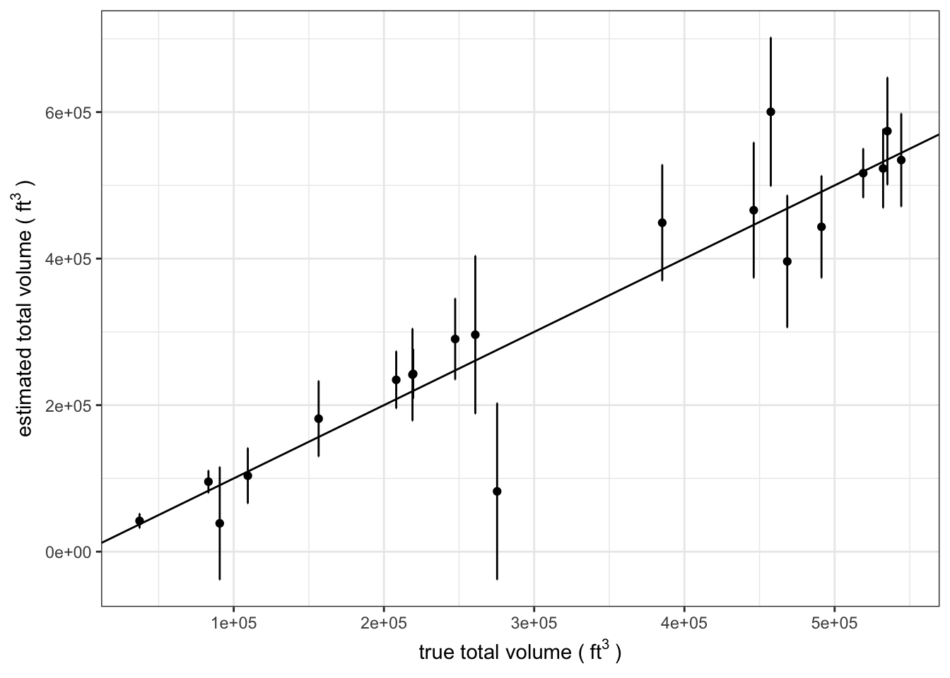
Population-level estimate
We can now combine the estimates from the primary sampling units to obtain an estimate of the population. To do this we will use the inclusion and selection probabilities to weight each sampled stand’s contribution to the population total.
Using the equations listed above we will compute estimates of the population total and sampling variance of that estimate, then convert those into estimates of cubic foot volume on a per-acre basis.
sampleSummary <- standDat %>%
  left_join(
    sampStands %>%
      select(id, pi_i, prop),
    by = "id"
  ) %>%
  ungroup() %>%
  nest() %>%
  mutate(
    var_I_syg = map(
      .x = .$data,
      .f = var_syg_wrap,
      y_var = tHat,
      pi_i_var = pi_i,
      id_var = id,
      jointProbs = jointProbs
    )
  ) %>%
  unnest() %>%
  summarize(
    totalCuft = sum(tHat / pi_i),
    fpcI = 1,
    fpcII = 1,
    varI = sum(var_I_syg),
    varII = sum(varTHat / pi_i),
    varTot = fpcI * varI + fpcII * varII,
    nObs = n()
  ) %>%
  mutate(
    seTot = sqrt(varTot),
    ci90Tot = qt(
      1 - 0.1 / 2,
      df = nObs - 1
      ) * seTot,
    meanCuft = totalCuft / totalAcres,
    seMeanCuft = seTot / totalAcres,
    ci90MeanCuft = ci90Tot / totalAcres,
    source = "estimate"
  ) %>%
  select(
    source, totalCuft, seTot, ci90Tot,
    meanCuft, seMeanCuft, ci90MeanCuft,
    nObs
  )

results <- bind_rows(sampleSummary, truth)
Results
Since we know the true population mean, we are able to compare the estimate from our sample of 20 stands to the truth!
results %>%
  ggplot(aes(x = source, y = meanCuft)) +
  geom_point() +
  geom_errorbar(
    aes(
      ymax = meanCuft + ci90MeanCuft,
      ymin = meanCuft - ci90MeanCuft
    )
  ) +
  ylim(0, max((results$meanCuft + results$ci90MeanCuft)) * 1.5) +
ylab(bquote("volume (" ~ ft^{3} ~ "/ac)"))## Warning: Removed 1 rows containing missing values (geom_errorbar).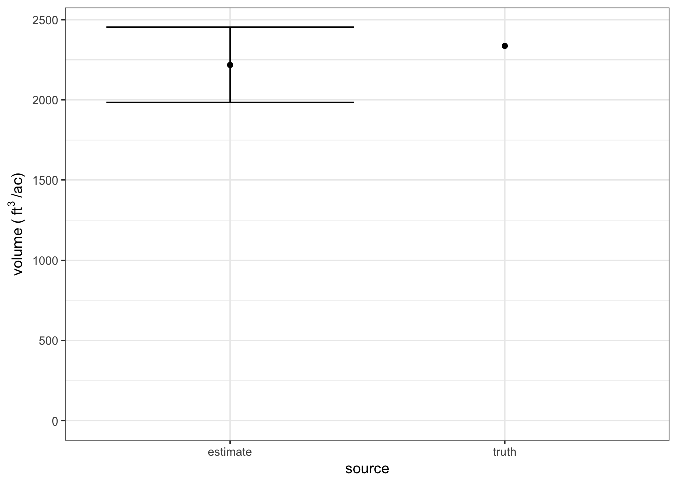
Simulate many samples
Though we may be stuck with it in real life, the result of a single sample is not very helpful for evaluating the performance of a sample design. To do that we will simulate many samples and evaluate the performance of various sampling intensities by assessing trends in precision and bias.
We are simulating 100 samples for six sample intensities: 10, 20, and 30 stands out of the 100 in the population. Stands will be selected using the same probabilities as the example we walked through earlier.
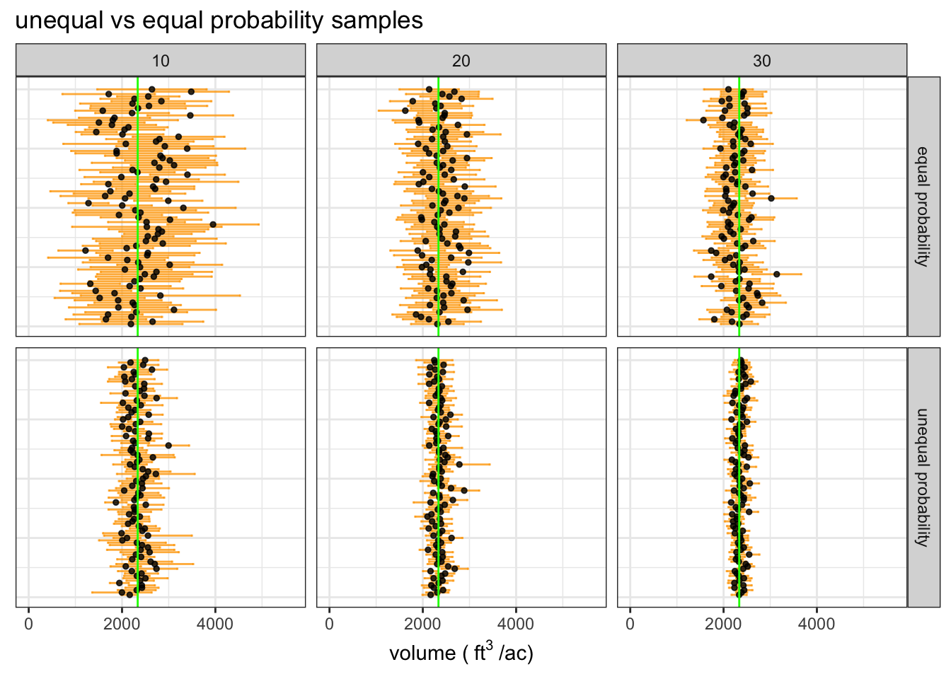
The plot of simulated sample means with 90% confidence intervals and the true population mean (green line) shows that each sample intensity yields accurate estimates and the precision of estimates increases substantially as we sample more stands.
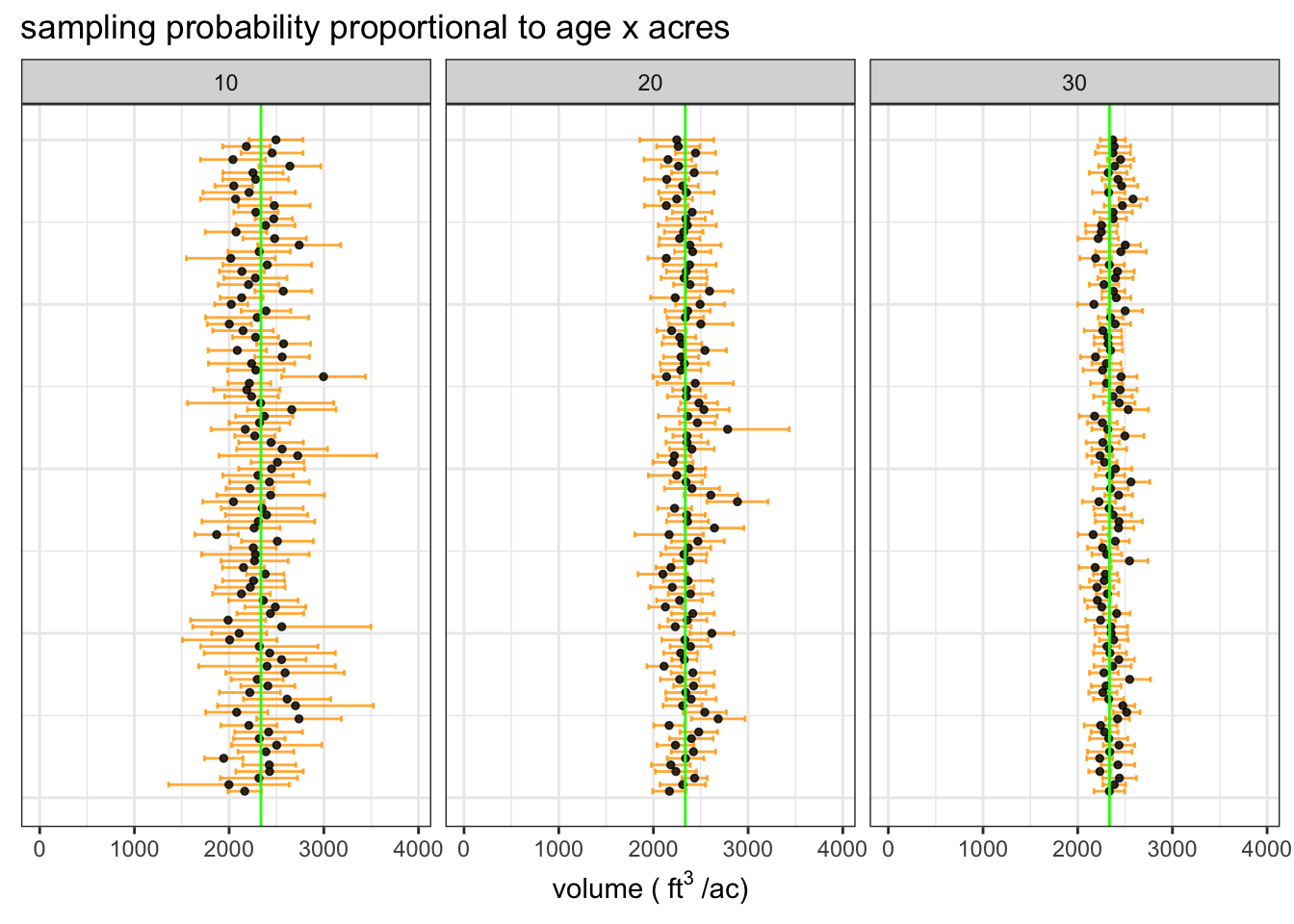
We expect ~90% of samples to yield a confidence interval that contains the true mean, this simulation gives the expected result. The results indicate that the half-width of the 90% confidence interval is about 10% of the mean when we sample 20 stands out of 100.
| source | # sampled stands | average sample cu. ft. per/ac | 90% CI | proportion of CIs containing true mean |
|---|---|---|---|---|
| estimate | 10 | 2324 | 373 | 0.94 |
| estimate | 20 | 2349 | 230 | 0.91 |
| estimate | 30 | 2350 | 167 | 0.93 |
| truth | - | 2336 | - | - |
Next, we are going to see how much more efficient the unequal probability sample is than a simple random sample for the first stage of sampling.
Simple random sample
To run the same simulation using a simple random sample we just need to make the sample weights equal for all stands. We can use the same Horvitz-Thompson estimators since the only things we have changed are the inclusion probabilities.
The simple random sampling yields mean estimates that are much less stable than the unequal probability sample, which is the expected result. The correspondingly wide confidence intervals reflect the reduced precision of the simple random sample.
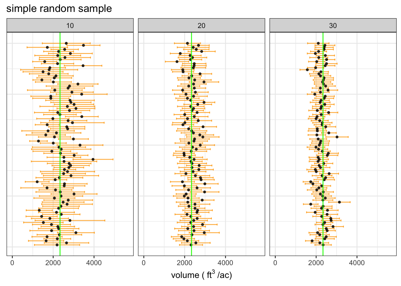
The wider confidence intervals reflect greater uncertainty in the estimate of the population mean. Notice that the proportion of CIs that contain the true mean is stil ~90%.
| source | # sampled stands | average sample cu. ft. per/ac | 90% CI | proportion of CIs containing true mean |
|---|---|---|---|---|
| estimate | 10 | 2372 | 974 | 0.88 |
| estimate | 20 | 2384 | 616 | 0.96 |
| estimate | 30 | 2276 | 439 | 0.92 |
| truth | - | 2336 | - | - |
We can see that the unequal probability sample yields much more stable estimates with higher precision. This demonstrates how we can save lots of time and energy with a bit of extra work during the sample design phase of a resource assessment project.
